This blog post is the 2nd and final part of my series of posts dedicated to providing a clear and practical step-by-step guide on how to use deep learning to carry out side-channel attacks—one of the most powerful cryptanalysis techniques. This post will walk you through how to train and use a TensorFlow model to recover an AES key from CPU power consumption traces.
Over the last three years, our research team at Google, in partnership with various research groups, has been working on developing deep-learning side-channels attacks (aka SCAAML Side Channels Attack Assisted with Machine Learning) and countermeasures to help build more secure trusted hardware. In our experience, everything becomes much clearer when you start writing code. That’s why we thought that the best way to help you get started in the exciting field of hardware cryptanalysis would be to provide you with a dataset, end-to-end code, and this practical guide that shows you, step by step, how to train and use a TensorFlow model to recover AES keys from a TinyAES implementation running on an ARM CPU (STM32F415) from its power consumption traces.
This tutorial is split into two parts due to the topic length:
-
Lightweight theory: The first part (my previous post) focuses on explaining the core concepts you need to know to understand how a deep-learning power-based side-channel attack works, what hardware and software setup you need to carry it out, and the advantages of using deep learning to perform an SCA (side channel attack) over traditional methods such as template attacks.
I highly recommend that you read it, if you haven’t done so already, as it explains the many concepts we will be using during the walkthrough.
-
Step-by-step recovery: The second post (this one) is a code walkthrough that explains, step by step, how to attack the TinyAES implementation running on an STM32F415 chip by training and using a Tensorflow deep-learning model. The SCAAML GitHub contains all the code, models, and the dataset you need to follow along and experiment.
If you prefer to watch a talk to learn the key concepts, Jean-Michel and I did a talk at DEFCON in 2018 on the subject. You can find the DEF CON slides here and the video recording here:
Overall, this walkthrough covers the following four topics in turn:
-
Setup: Where to get the code, models, and dataset you need to follow along and how the Github repository is structured
-
Preparing data: How to process power traces to create a dataset suitable to apply deep-learning (optional)
-
Training attack models: How to use our dataset to train the deep-learning models you will need to use to recover AES keys from power traces (optional)
-
Performing the attack: How to combine models and predictions to recover a full key out of the validation dataset
Note: As already mentioned, this tutorial assumes that you are familiar with the concepts and terminology discussed in the first part of this series. So, if there are concepts that are not clear as you follow along, take the time to look at the first part of the tutorial, as it likely has the answers you are looking for.
Environment setup
First things first: To get started, grab a copy of the code from Github and download the dataset we are going to be using throughout this tutorial. To make things easier and faster, in addition to the dataset and the attack code, we also provide you with the 48 pretrained models needed to attack all the attack points, so you don’t have to spend tens of GPU hours training them and can jump directly into the attack part if you wish.
Code

The code is available from the SCAAML Github under the Apache 2 license, so grab a copy of it, either by cloning the repo or downloading it.
The two directories you will need are:
-
scaaml/: This directory contains the SCAAML python library that we use for all the research we do around applying deep-learning to side-channel resilience. The key file we are going to discuss in-depth in this tutorial is the model file, which is under
scaaml/intro/model.py. It contains the TensorFlow Keras model architecture we are going to use to attack TinyAES. -
scaaml_intro/: This directory contains the code for this tutorial. As discussed in the README, there are two main scripts in this directory that we will use:train.pyto train the modelkey_recovery_demo.ipynbto perform the attacks with the trained models. As mentioned earlier, you can skip running train.py, as we provide trained models.
So, to install the code, you need to:
- Grab a copy of the code, either by cloning the repo or downloading it.
- Install the SCAAML package as discussed in the repo README.
Data
Once you have the code at hand, you need to download the TinyAES dataset and optionally the pretrained models from the Google Cloud Bucket. The easiest way to do so is to simply click on the links for those that are listed in the scaaml_intro/ README.
Important: Make sure you extract the archive in the right directories. The code assumes that the dataset will be in datasets/ and the models in models. Alternatively, you can change the code behavior, but that is out of the scope of this tutorial :)
Sanity check
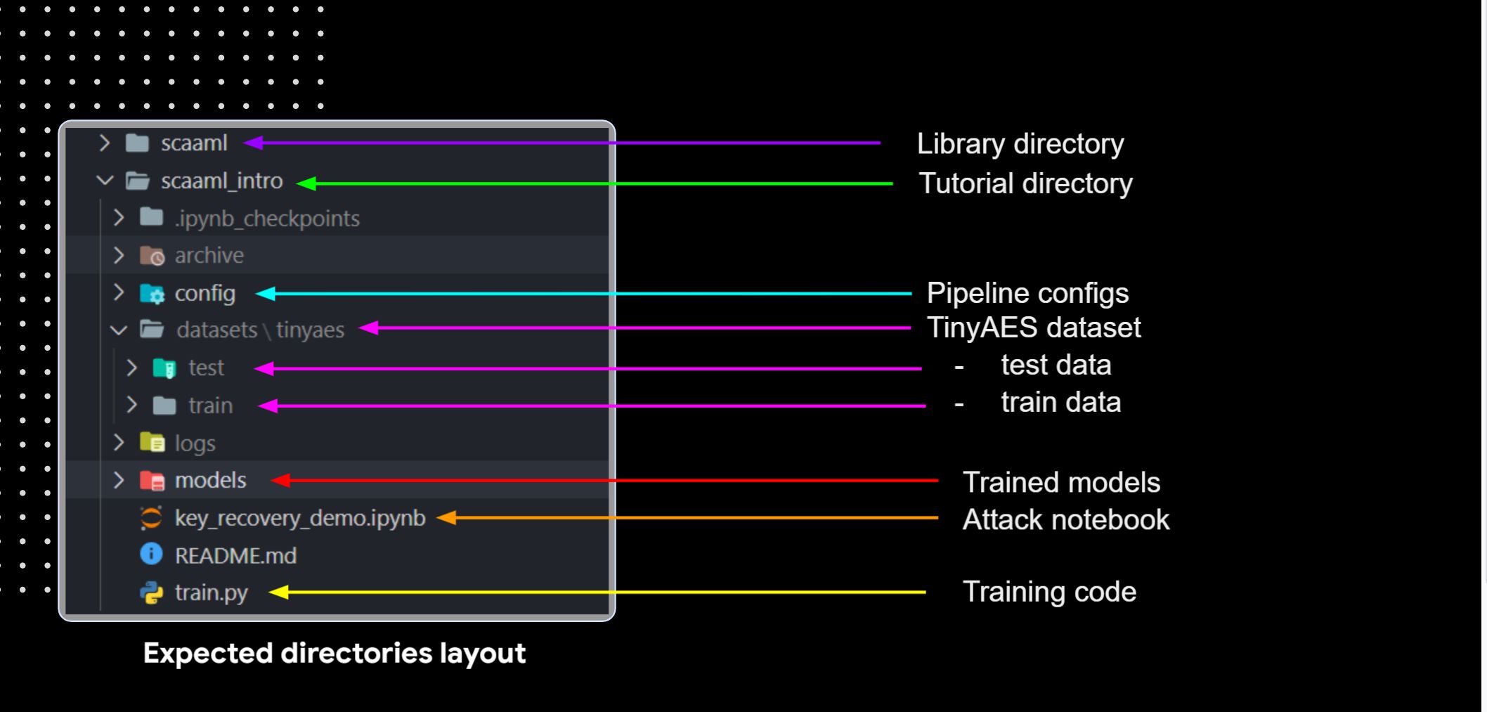
Once you are done installing SCAAML and extracting the tutorial data, you should have a repository that looks like the picture above. Double-check that the data is in the right place and that the SCAAML library is correctly installed to avoid errors moving forward.
Preparing the data
The goal of this step is to convert power traces into a dataset usable by machine learning. It includes three major operations:
-
Data mangling: We perform feature scaling to scale the power trace between -1 and 1. This is essential; otherwise most models won’t converge at all, as we discovered when we had a bug in our processing pipeline :( We also reshape the traces to add an extra dimension going from (batch_size, 20000) to (batch_size, 20000, 1). This extra dimension is needed to have a shape that is compatible with what the
Conv1D()layer expects.Conv1D()is the Keras 1D convolution layer. -
Compute attack points: For each trace, we precompute the expected sub_bytes_in and sub_bytes_out values. We also perform a matrix transpose to ensure that the data is of the form
[byte_id][example_id]as we want to be able to fetch values by byte_id as each model attacks a single key byte, as discussed in the first part of the series. Finally, we perform a categorical encoding of the byte value, as the model output will be a softmax over the 256 potential values. -
Package data as shard: Finally, we package the examples as shard, which contains all the examples for a given key value. This allows us to tune how many examples we want per key and ensure that the same key is not used in training and testing. It seems obvious that you should not use the same key both for training and testing, but I have seen datasets in the wild that do this, so storing data like this ensures that won’t happen to us. In our daily research, we use the TF.dataset format for our dataset, but this format is not straightforward to use, so for this intro tutorial, I converted the shards to the numpy format to make it easier for you to use and manipulate.
The code that produces the shards is not provided because it is part of a complex pipeline that is meant to scale to very large datasets (think >1T of traces) in TF.dataset format and run over Google DataFlow. There is no easy way for me to just “extract” the relevant part, so instead we provide the dataset already processed. Nevertheless, if you reimplement the data processing part, then you can test its correctness by using some of the dataset unit tests I wrote. They are located under /tests/scald/test_generator.py.
Training models

With the data at hand, it’s now time to train our models. The code used to train the model is located in train.py. It’s a fairly standard training code that takes as input a configuration file. Before explaining the interesting part of the training loop, let’s first discuss the config file structure and the model.py file, as you will need to understand this to understand how the training loop works.
Config file
The configuration file we will be using in this tutorial is stored in config/stm32f415_tinyaes.json. The reason we favor config-file-based training is for reproducibility purposes: It allows us to version the experiment and ensure that we can reproduce each experiment with its exact parameters. While, for the tutorial, it doesn’t matter, overall, configuration-based training is an important data-science practice that is worth applying every time, as it greatly improves reproducibility for the very slight overhead of parsing and maintaining a config file.
{
  "model": "cnn",
  "device": "stm32f415",
  "algorithm": "tinyaes",
  "version": "10",
  "attack_points":[ "sub_bytes_out", "sub_bytes_in", "key"],
  "attack_bytes": ["0", "1", "2", … , "14", "15"],
  "max_trace_len": 20000,
  "num_shards": 256,
  "num_traces_per_shard": 256,
  "batch_size": 32,
  "epochs": 30,
  "optimizer_parameters": {
    "lr": 0.001,
    "multi_gpu_lr": 0.001
  },
  "model_parameters": {
    "activation": "relu",
    "initial_filters": 8,
    "initial_pool_size": 4,
    "block_kernel_size": 3,
    "blocks_stack1": 3,
    "blocks_stack2": 4,
    "blocks_stack3": 4,
    "blocks_stack4": 3,
    "dense_dropout": 0.1
  }
}
Overall, as shown above, the config file is used to stipulate four things:
-
Hardware target: Define what is attacked using the
deviceandalgorithmfields. This is used by the code to know where to name/fetch the dataset, models, and logs in a consistent manner. -
What to attack: The
attack_pointsandattack_bytesfields define what to predict as output. As discussed in the first part of this series, there are three potential invertibleattack_pointsthat we can apply to the 16 bytes that make an AES 128 key. As a result, there are 3x16: 48 models that need to be trained overall.Note that the model performance across various bytes is roughly the same, so if you don’t intend to recover the full key and just want to play with the model architecture to see what works best, you can choose to test just a single byte at a time, knowing that the result will generalize well. This is what we do when we develop/refine our model architectures.
In terms of
attack_points, you can skip thekeyattack point, as it doesn’t work if you want to save time. Targeting the fieldsub_bytes_inorsub_bytes_outwill give you roughly equivalent performance. -
How much data to load: This is defined with
num_shardsandnum_traces_per_shard. As discussed earlier, one shard contains all the examples for a given key, so the number of shards is equivalent to the number of keys to use. Thenum_traces_per_shardrepresents how many distinct power traces/plaintext samples to use for a given key. Given that our data sampler is designed to uniformly sample the key and plaintext bytes at capture time using 256 shards x 256 examples (65536 examples total) should be enough to cover all keys/plaintexts pair values for a given key byte and will be enough to reliably recover the validations keys .Note that the data loader provided with the tutorial does not check for uniformity and just loads the n first shards—it’s not a problem here, but certainly not what I would recommend for more rigorous attacks and research.
-
Model configuration: The rest of the file, as discussed below, allows us to specify how to configure the model architecture. For research, using configuration-based models is essential, because it allows you to perform architecture search via hyper-tuning. For this, we use Keras Tuner, which was initially developed for this exact purpose before taking on a life of its own and becoming a core element of the TensorFlow / Keras ecosystem.
What the model parameters mean will be discussed in the next section.
Note that there are two different learning rates specified in the file. This is because the code relies on tf.distribute.strategy to distribute over multi-GPU, which requires you to increase the size of the
batch_sizelinearly in the number of GPUs. If you are not familiar with multi-GPU training, don’t worry! I will highlight how we use Tensorflow distribution strategy in practice when walking you through the train loop.
Model architecture
As model architecture, we are going to use a residual convolutional architecture, as it provides good performance while training quickly. It should take less than 30 minutes to train a model (~24 hours for the 48 models) on a fairly recent GPU (20xx/30xx/ P100/v100/T4).
The model architecture is defined in the file scaaml/intro/model.py and uses the Keras Functional API. For those who aren’t familiar with it, the Keras functional API allows you to define models with nonlinear topology, which is essential if you want to do shared layers, multiple inputs, and multiple outputs. If you are serious about deep-learning and TensorFlow, then learning how to use this API instead of the sequential one is a must.
General structure
inputs = layers.Input(shape=(input_shape))
x = inputs

# stem
x = layers.MaxPool1D(pool_size=pool_size)(x)

# trunk: stack of residual block
for block_idx in range(4):
  filters *= 2
  x = stack(x,
        filters,
        num_blocks[block_idx],
        kernel_size=block_kernel_size,
        activation=activation)

# head model: dense
x = layers.GlobalAveragePooling1D()(x)
for _ in range(1):
  x = layers.Dropout(dense_dropout)(x)
  x = layers.Dense(256)(x)
  x = layers.BatchNormalization()(x)
  x = layers.Activation(activation)(x)

outputs = layers.Dense(256, activation='softmax')(x)
Overall, our model, depicted in the code above, is based on the preactivation version of the ResNet architecture (aka V2). While testing, it became clear that this version, which puts the activation before the convolution appears to work better than the other resnet variants for our use-case. There are a few key differences between our model and the traditional ResNet architecture:
-
Our model uses
Conv1D(): We are dealing with time series (batch_size, trace_len, value), not images (batch_size, width, height, channels), so our data shape is different (1D rather than 2D) and, therefore, we need to use the appropriate layers for this type of shape. -
Our model starts with
layers.MaxPool1D(pool_size=pool_size)(x)because our capture was oversampled (as explained in the first post), so starting with a max pool is a sensible way to make our model smaller and converge faster. Its size is controlled with theinitial_pool_sizeparameter in the config. Additionally, we don’t use an initial convolution layer, because we use the preactivation version (more on this later). -
We use a simplified “stack” of convolution growing functions, where each stack simply doubles the number of filters from the previous one. That makes for a simpler loop and reduces the number of hyper-tuning parameters. I will describe the stack structure in the next section.
The head of the model is fairly standard; we have a Dropout() to help generalize followed by a dense block where the Dense() layer with its Activation() layer is intertwined with a BatchNormalization() layer to speed up convergence. I tend to favor having the batch normalization layer between the dense layer and its activation layer, even though there is a lot of debate over whether it’s the optimal way to order the layers or not. Finally, I did hard code to use only a single dense block, because that is all you need for most SCAAML attacks.
Last but not least, our output layer is as expected, a Dense(256) layer with a softmax activation. It has a size of 256 because a byte has 256 potential output values and we encoded the data in a categorical function, as explained in the initial blog post. The softmax is needed to normalize the output.
Stack structure
x = block(x,
      filters,
      kernel_size=kernel_size,
      activation=activation,
      conv_shortcut=True)

for i in range(2, blocks):
  x = block(x, filters, kernel_size=kernel_size, activation=activation)
x = block(x, filters, strides=strides, activation=activation)
return x
The core of the model is stacks of residual blocks, and the code, shown above, starts at line 81 in the model file. Overall, the code is fairly straightforward: Each stack includes at least 4 blocks, like the standard ResNet. Increasing the number of blocks is what allows us to vary the “computing power” of the network by increasing its depth. With the ResNet architecture, you mostly want to increase the number of blocks in stacks 2 and 3, and leave stacks 1 and 4 at 3 blocks—see the original research paper or reference implementation for more detail.
It’s worth mentioning that the first block uses conv_shortcut. This is needed to normalize the shape coming from one stack to another but should be avoided otherwise.
Residual block structure
The core of our network consists of preactivated residual blocks that are implemented starting in line 22, shown below. The preactivation version means that we start with a batch normalization and do the activation before doing the convolution. I think the reason the preactivation works better for our use case is that it greatly helps the network to start by reducing the covariance using the batch normalization. Overall, in our experience, whichever architecture we use, in most cases the batch normalization really helps models’ convergence.
Additionally, as mentioned earlier, the main difference with the standard version is that we use Conv1D() layers instead of Conv2D() layers because we deal with time series.
Besides those two points, there is not much to add; the model is a textbook residual architecture. It’s a good architecture for SCAAML attacks because the residual connections greatly reduce vanishing gradient issues, which is a major issue when using deep-learning for SCA.
x = layers.BatchNormalization()(x)
x = layers.Activation(activation)(x)

if conv_shortcut:
  shortcut = layers.Conv1D(4 * filters, 1, strides=strides)(x)
else:
  if strides > 1:
    shortcut = layers.MaxPooling1D(1, strides=strides)(x)
  else:
    shortcut = x

x = layers.Conv1D(filters, 1, use_bias=False, padding='same')(x)
x = layers.BatchNormalization()(x)
x = layers.Activation(activation)(x)

x = layers.Conv1D(filters, kernel_size, strides=strides, use_bias=False, padding='same')(x)
x = layers.BatchNormalization()(x)
x = layers.Activation(activation)(x)

x = layers.Conv1D(4 * filters, 1)(x)
x = layers.Add()([shortcut, x])
return x
Training loop
The training loop, located in the scaaml_intro/train.py, while fairly straightforward, includes a few interesting tidbits that are worth discussing.
Data generators
Instead of passing the dataset directly to the model, we use generators, which essentially wrap the tf.data.Dataset.from_tensor_slices() API while selecting the correct output value (Ytrain) based on the requested _targeted_byte _and _attack_point. The wrapper also converts the output value to its categorical representation. We do the to_categorical() on the fly to save disk space by storing the values as uint8.
For the demo, using tf.data.Dataset is not necessary because the dataset is very small, however I decided to still use it because it is what we use in our research pipeline and I wanted the tutorial to be as close to the real thing as possible.
The reason we use this approach in our research is because it’s the most efficient (albeit a little painful and quirky in my experience) way to feed data to a Tensorflow model and scale up to TB scale datasets using the TFRecordDataset format (which is what we do).
An important gotcha with this approach, which is due to the fact that we store all the examples for the same key in the same shard, is that you need to have a large shuffle window for your dataset. We use a window of 65535 to ensure that the batches contain a good mix of various key values. Not properly shuffling data results in the models not converging properly. The relevant code is in scaaml/intro/generator.py at line 70/76:
# make it a tf dataset
cprint("building tf dataset", 'magenta')
dataset = tf.data.Dataset.from_tensor_slices((x, y))
dataset.cache()
if is_training:
  dataset = dataset.shuffle(shuffle_size, reshuffle_each_iteration=True)
dataset = dataset.batch(batch_size).prefetch(tf.data.experimental.AUTOTUNE)
return dataset
Multi-models
The loop train multiple model sequentially covers all the requested attack points and bytes, which is why the training loop is made of two loops:
for attack_byte in config['attack_bytes']:
  for attack_point in config['attack_points']:
Multi-GPUs
To use multiple GPUs, you need to multiply the batch_size by the number of GPUs. This is done during the setup phase of the code in line 34. The get_num_gpu() function is simply a wrapper around the [tf.config.list_physical_devices()](https://www.tensorflow.org/api_docs/python/tf/config/list_physical_devices) that counts how many GPUs are available.
BATCH_SIZE = config['batch_size'] * get_num_gpu()
The other part of multi-GPU is to use the TF.distribute.MirroredStrategy() API, which is the standardized way to do distributed training in TensorFlow 2.x. This is done in the code at line 75/76 by initializing the strategy and then building/training the model under the strategy scope as follows:
# multi gpu
strategy = tf.distribute.MirroredStrategy()
with strategy.scope():
  model = get_model(input_shape, attack_point, config)
…
  model.fit(g_train, ….)
Running the train loop will result in the models being saved in the scaaml_intro/models/ directory. The models are saved, as usual, via the [ModelCheckpoint()](https://www.tensorflow.org/api_docs/python/tf/keras/callbacks/ModelCheckpoint) callback to ensure that we save the best possible state.
Recovering test keys

Now that we have our models trained, it is time to use them to recover our evaluation keys that were not used during training. The code to do so is available in the Jupyter notebook scaaml_intro/key_recovery_demo.ipynb. The notebook is heavily documented, so instead of paraphrasing the existing explanations, I am going to use this final part as an opportunity to tie everything that has been discussed in the two posts together, to give you a cohesive picture of how the attack works end to end and leave you with a good understanding of what SCAAML attacks are, and how to perform them.
Setup
From cells 1 through 5, we start by setting up our environment. There are three attack points for AES that can be used to recover the key used for encryption, and each model is trained to predict the attack point value for a specific byte, which means that we have 48 models in total, as AES 128 uses, unsurprisingly, a 16-byte key: 3 attack points x 16 bytes = 48 models.
This is why, in cell 4, we group models by attack point and verify that we have all of them, because we are going to combine the output of the 16 models, targeting the different bytes, to recover the full key. From training the models, we know that attacking TinyAES using the key attack point is not working, as the model’s accuracy stays at 0.004, which is the random baseline: 1/256 = 0.004. This leaves us with targeting either sub_bytes_out or sub_bytes_in, which will both work, given that TinyAES protects neither.
Single byte recovery
We start by recovering a single byte before we scale up to the entire key. The first thing to do is load our model (cell 6) and then, for each shard that represents a different key, we try to predict the value of the attack_point for the targeted byte (cell 7).
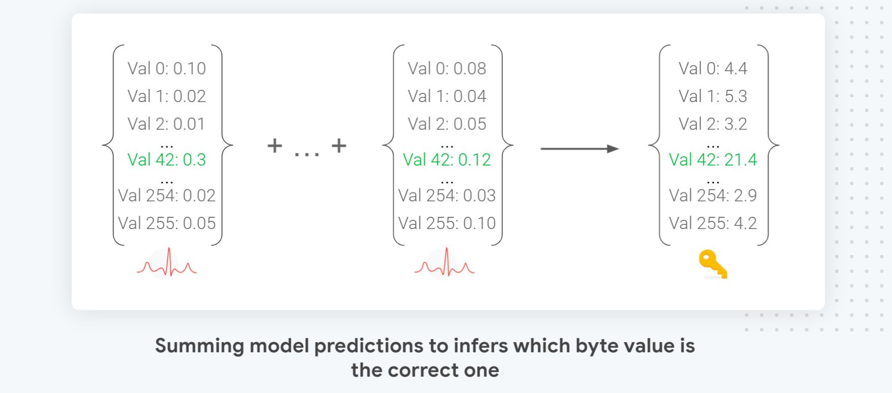
As our model uses a softmax output, combining the prediction results on different traces is as simple as accumulating the probabilities as illustrated in the figure above. Note that we sum the logarithm to avoid numerical errors: vals = vals + np.log10(kp + 1e-22)
Model generalization
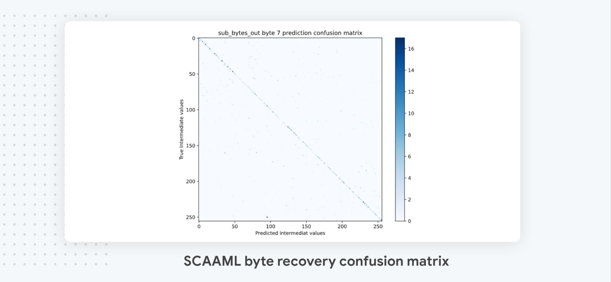
We can check that our model generalizes well across all possible intermediate values by plotting the confusion matrix** (cell 9)** and checking that we have a nice diagonal. This is an important step because, in our experience, sometimes models collapse and predict the single value 0.
Recovery performance
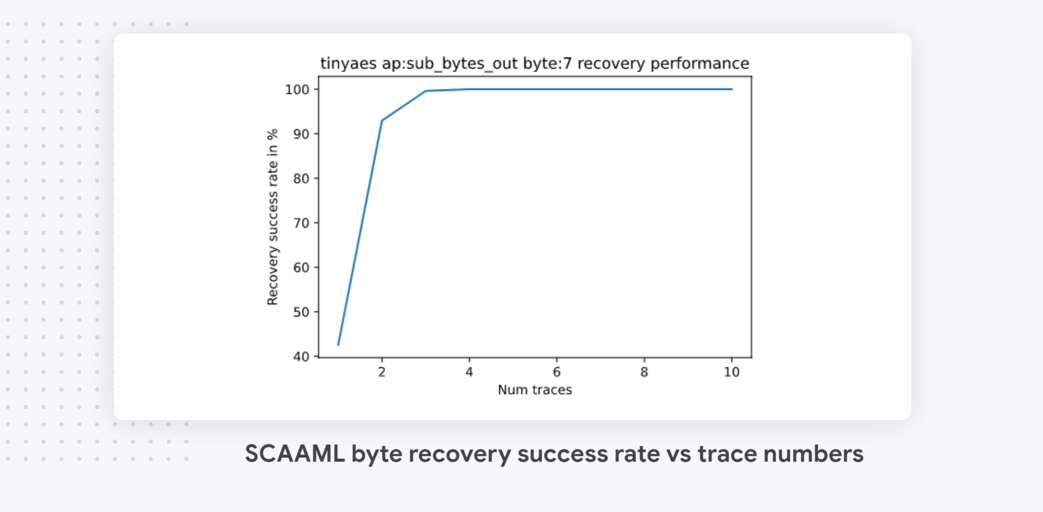
As our model accuracy is better than random, accumulating trace predictions will ultimately ensure that the predicted byte value with the highest score will be the correct one (Condorcet’s jury theorem). TinyAES not being protected, our model has a high accuracy (45% as reported in cell 8), which means that only a few traces are needed to recover the correct byte values for the 256 test keys, as illustrated in cell 10. As shown in the chart, reproduced above, with even 2 traces we can recover over 90% of the correct values. On the most protected implementations, you usually won’t get a 100% recovery rate unless you use an inordinate number of traces.
As mentioned in the first part of the series, there are many metrics you can use to evaluate the efficiency of an attack. In **cell 11, **the notebook showcases** **how you can compute some of the major ones, giving you:
- The minimum number of traces needed to recover a byte, which is the worst case scenario for the implementation.
- The maximum amount of traces needed to recover all the keys, which is the best case scenario for the implementation.
- The AUC (area under the curve), which is a cumulative performance metric that is super helpful to compare performance across implementation and attack techniques, as it’s a single score that measures how “fast” the bytes can be recovered. A score of 1, the perfect score, means you can recover everything with a single trace.
Full key recovery
Recovering a full key is a matter of selecting a target shard (cell 12) and then iterating through the 16 trained models to recover its byte one at the time, as illustrated in **cell 13. **The loop is fairly straightforward: You load a model, predict the values, sum them, and take the best one.
When done looping, all is left to do is to display the results to show that, indeed, the right key was recovered. This is done in **cell 14. **The loop takes a few minutes, so to make the wait more bearable without going crazy on the UI, I used tqdm’s ability to add an arbitrary suffix to the progress bar to show bytes as they were recovered.
Wrap-up
The successful recovery of a full AES key using the deep-learning models we trained concludes our guide, as you now have, hopefully, all the elements you need to get started. There are many ways the attack could be improved and many avenues to explore, but this guide is already very long (over 50 pages), so we will explore those at a later stage, when I will talk about our research results.
Thank you for reading this post till the end! If you found this guide useful, please take a moment to share it with people who might find it interesting too. I spent over a hundred hours creating this content, and what kept me going is the hope that it would be useful to our community, so having it shared and used really means a lot to me.
To get notified when my next post is online, follow me on Twitter, Facebook, or LinkedIn. You can also get the full posts directly in your inbox by subscribing to the mailing list or via RSS.
🙏 A big thanks to Celine, Francois, Emmanuel, Jean-Michel, Remi, Fabian and the insider community for their invaluable and tireless feedback - couldn’t have done it without you!
A bientot 👋


