This blog post series provides a practical step-by-step guide to using deep learning to carry out a side-channel attack — one of the most powerful cryptanalysis techniques. We are going to teach you how to use TensorFlow to recover the AES key used by the TinyAES implementation running on an ARM CPU (STM32F415) from power consumption traces.
Hardware-backed encryption is the cornerstone of system security. From operating systems’ trusted boots, to phone data encryption, to fingerprint storage, to credit card chip, to Bitcoin hardware wallets used for cryptocurrency storage (e.g Bitcoin), hardware-backed encryption is used everywhere to secure secrets.
Over the last three years, our research team at Google in partnership with various research groups has been working on developing deep-learning side-channels attacks (SCAAML) and countermeasures to help build more secure trusted hardware. In our experience, everything becomes much clearer when you start writing code. That’s why we thought that the best way to help you get started in the exciting field of hardware cryptanalysis would be to provide you with a practical guide that shows you, step by step, how you can recover AES keys from a real hardware target by training a TensorFlow model on CPU power traces.
The overall plan is for the guide to be split into two parts due to the topic length:
-
Lightweight theory: The first part (this post) is dedicated to explaining the core concepts you need to know to understand how a deep-learning power based side-channel attack works, what hardware & software setup you need to carry it out, and a short explanation of the advantage of using deep learning to perform a SCA (side channel attack) over traditional methods such as template attacks. It’s a fairly long post (>5800 words), but there are a lot of concepts you need to bring together to get such attacks to work and understanding how everything fits together is one of the main difficulties to get started in hardware cryptanalysis. This is why I did my best to strike the right balance between keeping it brief and providing you with enough explanation and examples so it’s clear how a side-channel attack works. The depth and length also explains why it took me over two years to write a guide that I was happy with since we did our initial side-channel attack talk using deep-learning at DEF CON 😊
-
Step-by-step recovery: The second post is a code walkthrough that explains, step by step, how to attack the TinyAES implementation running on an STM32F415 chip by training and using a Tensorflow deep-learning model. The SCAAML GitHub contains all the code, models, and the dataset you need to follow along and experiment with. Note that without understanding the concepts discussed in this post, it will be hard for you to make sense of this part, so I encourage you to read this post first, all the way to the end, even if it is a little long. 😊
If you prefer watching a talk to learn the key concepts, Jean-Michel and I did a talk at DEFCON in 2018 on the subject. You can find the DEF CON slides here and the video recording here:
Finally, if you would like to jump straight to the code used in this guide, then head out to the SCAAML GitHub tutorial section.
To get started on our journey, this post will provide you with the needed background by covering the following topics in turn:
-
What is a side-channel attack (SCA)? A short introduction about what side-channel attacks are and what type of information they exploit.
-
SCA main applications: Briefly covers what side channels are used for and some of their main applications.
-
SCA brief and incomplete history: How side channels came into existence and evolved, from being used during the Cold war (TEMPEST) to spy on communication, to recovering an RSA crypto key to attack a modern CPU (Spectre).
-
Deep learning in a nutshell: What is deep learning? How do you train a deep neural network? And, how does doing so relate to side-channel attacks?
-
Why use deep-learning for SCA? What are the main advantages of using deep-learning SCA instead of traditional SCA?
-
Differential power analysis side-channel attack (DPA) overview: Explanation of the various steps needed to carry out side-channel attacks that exploit power consumption variations.
-
SCA collection phase: A delve into the power trace collection process, including what hardware to use and how to sample data.
-
SCA training phase: Discussion of which part of the algorithm to attack (attack point) and how to design your neural network for this.
-
SCA attack phase: How to combine your model prediction to recover key bytes and how to measure success.
If you are familiar with any of those topics, like how deep-learning works, feel free to skip to the next section, as they are designed to be (mostly) independent from each other.
What is a side-channel attack?

A side-channel attack is an implementation specific attack that exploits the fact that using different inputs results in the algorithm implementation behaving differently to gain knowledge about the secret value such as a cryptographic key used during the computation using an indirect measurement such as the time the algorithm took to execute the computation.
One of the most infamous cases of timing attack, is the fact that the time taken by the naive square-and-multiply algorithm used in textbook implementation of the RSA modular exponentiation depends linearly on the number of “1” bits in the key. This linear relation can be exploited by an attacker, to infer the number of “1” bits in the key by timing how long it takes to perform the computation for diverse RSA keys. He can then use this knowledge to guess the number 1 in an unknown RSA key stored in a hardware crypto device by simply measuring how long the code takes to run. While nowadays most hardware crypto-implementation have constant time implementation, timing attacks are still actively used, mostly in blind SQL injection.
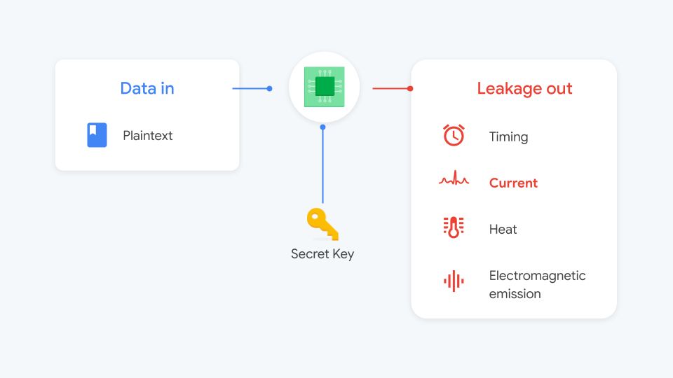
More generally, you can think of a side-channel attack as any attack that exploits indirect measurements of a computation via an auxiliary mechanism to recover a secret value (usually a cryptographic key). Popular indirect measurements include the power used during the computation (power analysis attacks), the time the computation took (timing attacks), and the electromagnetic emissions (EM attacks) generated. In practice, to recover a key, you need many repeated indirect measurements where you vary the inputs combined with careful computation (or deep-learning!) to recover the secret key used during the computation or what was displayed on the screen.
Side-channel attacks main applications

First and foremost, side-channel attacks are one of the most effective ways to attack secure hardware, such as cryptocurrency hardware wallets, because instead of attacking the cryptographic algorithm itself, which is often well secured, side-channels target the algorithm implementation, which is less scrutinized. Implementing algorithms in a way that leaks no information is extremely hard. You not only need to make it time constant, but also need to obfuscate every side effect of loading/unloading data in the physical memory, which requires implementing complex software and hardware countermeasures.
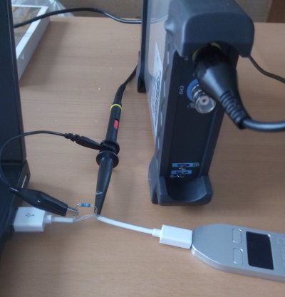
Doing all this while maintaining reasonable production cost and good performance is next to impossible. For example, in 2015, Jochen Hoenicke was able to recover the private key of a Trezor hardware bitcoin wallet, using a power side-channel attack. More generally, the security community generally agrees that it is indeed possible to recover secret keys from almost any implementation, even if the algorithm itself is secure, thanks to side-channel attacks.
The only question is, how much effort does such an attack require? This is what crypto-chip certifications measure: the cost and skill set needed by an attacker to recover secret keys. The higher the certification, the more expensive it would be for the attacker to recover the key of a given device. The more valuable the key is, the higher the certification level must be, and the more expensive the hardware is due to the cost of developing and implementing countermeasures.
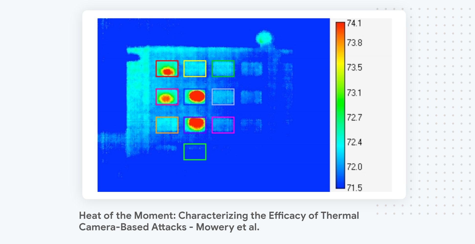
In addition to recovering secret keys, side-channel attacks have been extensively used to attack systems where the output of the computation is not visible to the attacker. The most famous and widespread use of side-channel attacks in that context are Blind SQL injection attacks. Other creative use cases include using an acoustic side-channel to recover the content that a printer printed or using thermal imaging to recover a pin code.
Side-channels: a brief and incomplete history
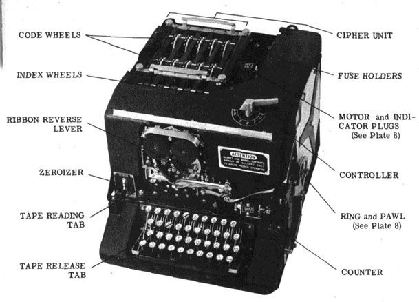
Contrary to popular belief, which ties the development of side-channel attacks to the Cold War (circa 1950), an NSA document called “TEMPEST: a signal problem” was declassified in 2008. This document reveals that the earliest side-channel attack was, in fact, discovered by a Bell Lab engineer as early as 1943. The document reveals that this engineer discovered that every time someone was encrypting a message on the SIGABA teletype encryption machine, visible in the screenshot above, a distinct spike was visible from afar on an oscilloscope located in another part of the lab. Through careful analysis, he figured that it was possible to use those spikes to recover the plaintext that was typed on the teletype. The side-channel and TEMPEST program was born.
Side-channel rose in popularity in academic circles in 1996, when Paul Kocher demonstrated how to recover private keys using a timing attack, in his seminal paper “Timing attacks on implementations of Diffie-Hellman, RSA, DSS, and other systems.”. Three years later, he popularized the use of power-consumption-based side-channel attacks in a paper simply named: “Differential Power Analysis”.

Fast forward to 2017, when side-channel attacks hit the hardware mass market with the disclosure of the Spectre vulnerability for Intel CPU, and its numerous follow-ups, which exploit CPU side-channel attacks. In a nutshell, they trick the CPU speculative execution engine into accessing private data by causing branch mispredictions on the targeted memory address and reading the memory values using a timing attack.
Deep learning in a nutshell
Before delving into how to perform a power analysis side-channel attack, let’s briefly summarize what deep learning is and how you train and evaluate a deep-learning model. You will need to know this to understand how the training and evaluation phase of a side-channel attack works when you rely on a model to perform the attack.
What is deep learning?
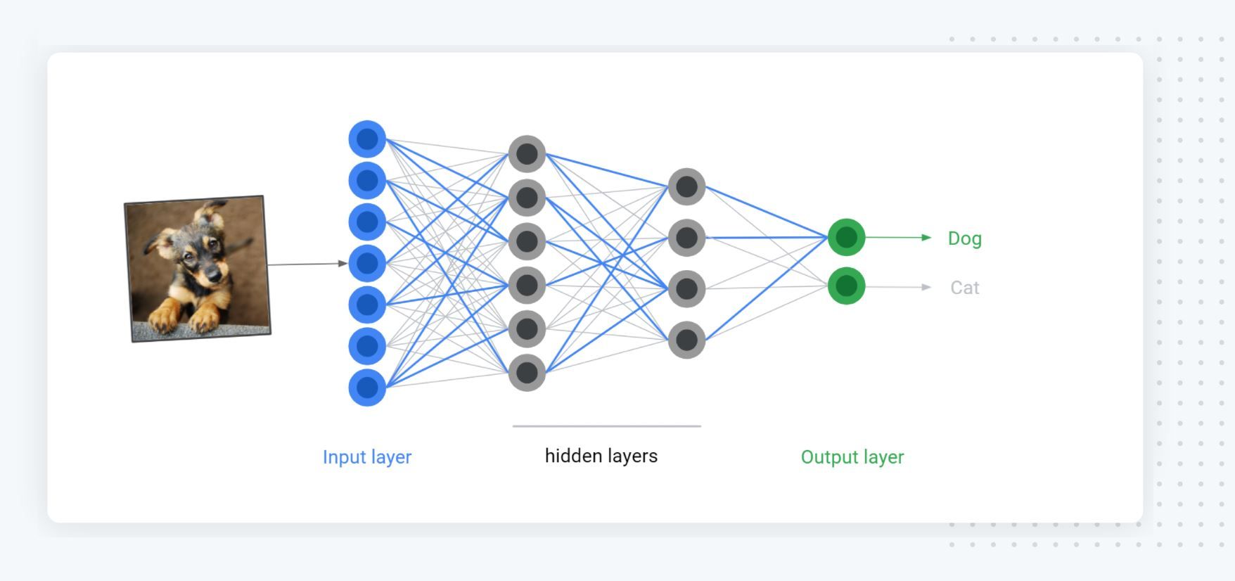
At its core, deep learning is the broad family of techniques that uses deep artificial neural networks. Inspired by biological neural networks, artificial neural networks are computing systems made of (virtual) neurons organized in layers. A neural network is made of interconnected layers stacked like pancakes to give the network the ability to extract higher-level representations of the data and perform complex computations on them. We commonly call modern neural networks DNN (deep neural networks) because modern networks routinely stack hundreds of layers.
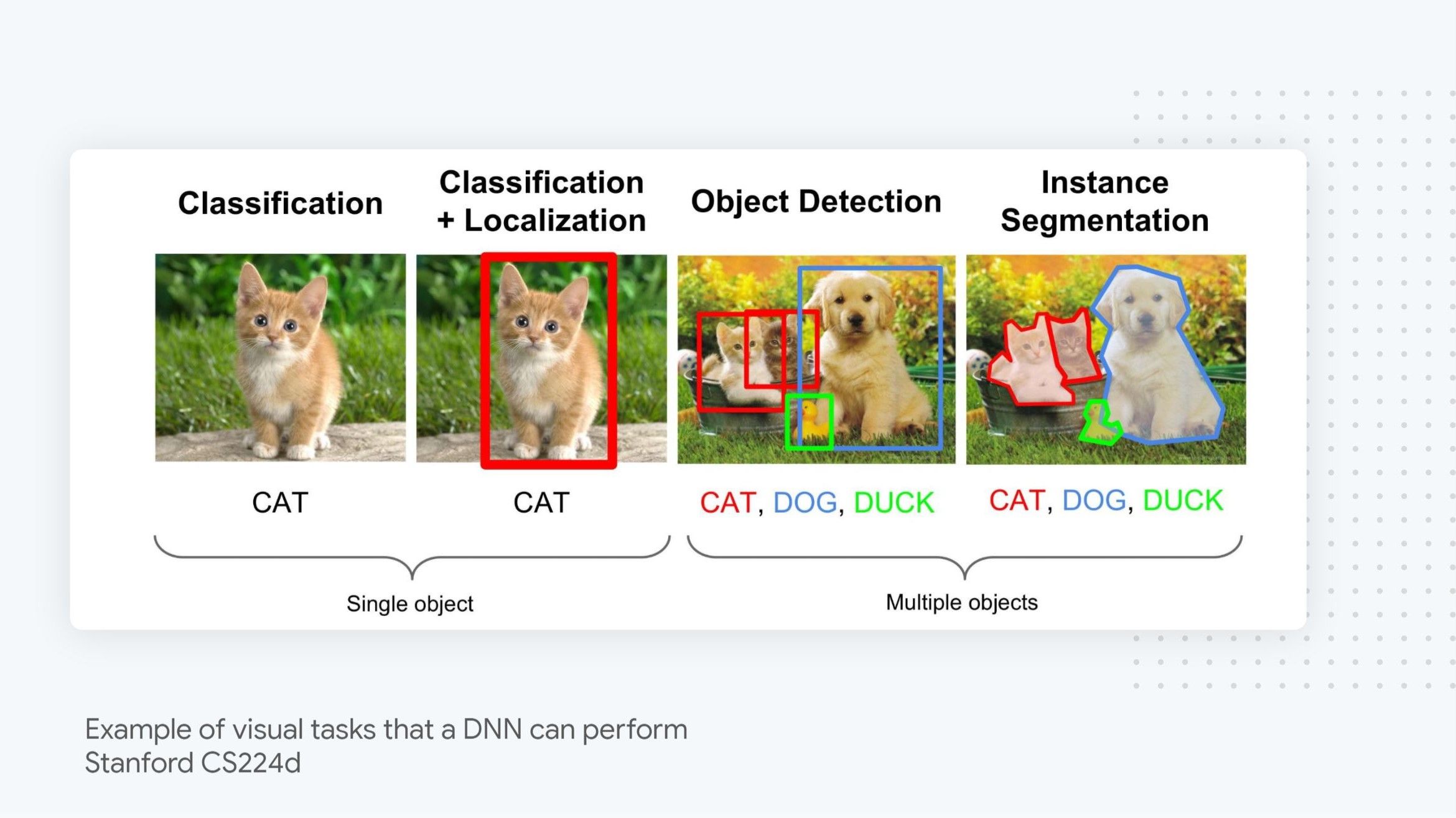
Due to their computational power, DNN are universal approximation functions, which means that with enough data, capacity, and computation time, they are able to learn to approximate many interesting functions, such as finding all the objects present in an image by looking at the image’s raw pixels, deciding how to drive a car based on the car sensor output, generating realistic speech (an audio wave) from user-supplied text, and translating text from one language to another.
Depending on the task at hand, we use a model architecture that exhibits different tradeoffs and benefits. For side-channel attacks, we mainly use 1D convolution neural networks (CNN) and recurrent neural networks (RNN), as they are well suited to process time series data.
How to train a DNN
You teach DNN to perform a given task, such as recognizing what is depicted in an image, by providing it with many examples of what you want it to do. For our image recognition case, you supply it with many diverse images (inputs) and their associated labels (output) as training data. During the training phase, those pairs (inputs/outputs) are repeatedly “shown” to the network. For each pair, the network outputs what it thinks the correct answer is (forward pass), and after every few images (batch), the stochastic gradient descent method is used to correct the network inner-values called weights based on the mistakes it made (back propagation pass).
Over time, thanks to this feedback loop, the number of mistakes decreases and the network becomes more accurate. As the network reaches its peak performance, we say the network has converged (aka it has learned how to predict the correct outputs). The better the model/training process is, the more accurate the network is. Accuracy being essentially how many answers the model got right.
To get a better sense of how this training process works, you can train your own DNN to recognize things directly in your browser by heading to the teachable machine site.
How does this relate to side-channel attacks?
For side-channel attacks, we follow this exact training process by feeding the power traces as inputs to the network and training the network to predict the key byte or an intermediate value that allows recovery of the key byte as output, as discussed later in the post.
Why use deep learning for SCA?
Overall, as illustrated in the rest of the post, using deep learning for SCA provides three major advantages:
-
Working directly on raw data: Models learn directly from the raw power consumption or electromagnetic traces instead of relying on human-engineered features and assumptions. This makes attacks simpler to design, reduces the need for domain-specific expertise, and, in the long term, will likely lead to more efficient attacks, the same way it did for computer vision applications. In particular, unlike the traditional attack techniques, you don’t need to resynchronize the traces or perform feature selection.
-
Direct attack point targeting: Models can learn to directly predict targeted intermediate values without using approximate models. Similarly to the first point, this simplifies the attack design and ultimately makes it more flexible and more efficient.
-
Natural Probabilistic attack: Last but not least, models’ predictions, as discussed below, can be used to mount an efficient probabilistic attack as the model output scores on multiple power traces can be directly combined to rank every possible byte value from the most likely correct to the least likely.
Power based side-channel attack overview
Now that we know what side-channel attacks and deep learning are, it is finally time to delve into how to combine them to recover AES keys from trusted hardware by looking at power traces.
Overall, a power based side-channel attack is a side channel that looks at how power consumption varies during a computation (e.g encryption) to infer what values (e.g AES keys) were supplied to the computation. Like most side-channel attacks, it is a known plaintext attack, where the attacker controls the plaintexts fed to the encryption device but has no control over the key.
The goal of a power-based side-channel attack is to learn how to tie specific power consumption patterns (input) to a given crypto key byte value being used during the computation (output).
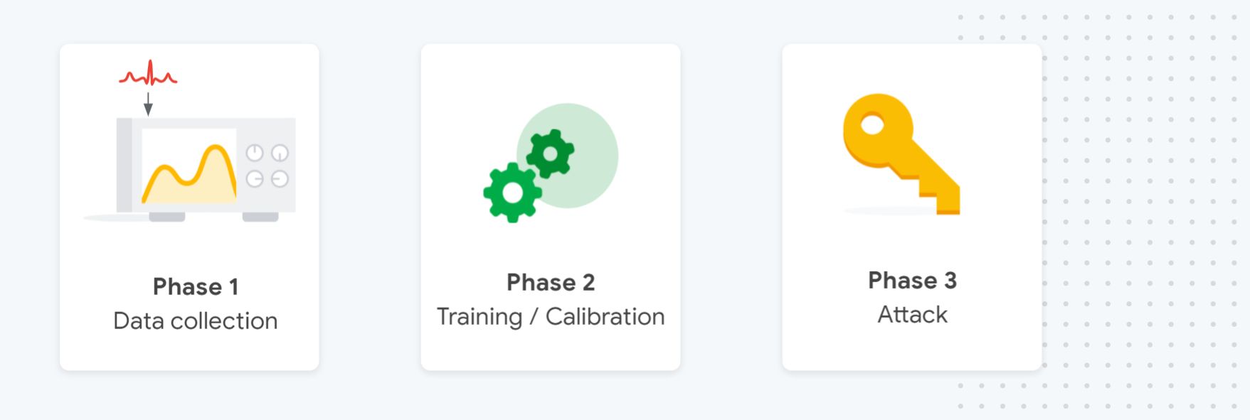
The attack has three main phases: First, we have the data collection phase, during which a data set of traces is collected,.Then, we have a training phase, in which the attacker calibrates the template (classic attack) or trains the machine-learning model.
Finally, there is the attack phase,where the template/model is used to recover a set of secret keys and evaluate the implementation resilience to SCA. For each key attacked during this phase, the attackers use multiple traces and combine their probabilities to make the best guess possible.
An important and often overlooked technical aspect of this type of side channel attack is that It won’t recover the key in one go; instead, the attack focuses on recovering a single key byte. This is why for AES128 you need 16 attacks (and 16 models) to recover the whole key.
Now that we have a better sense of how the attack works overall, Let’s delve into how each of the three phases works in detail.
Collecting power traces
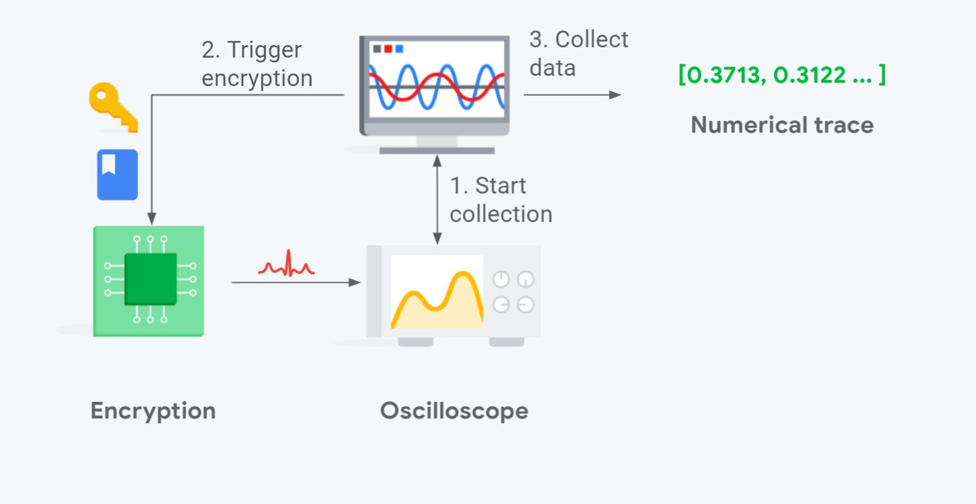
As outlined in the diagram above, capturing power traces roughly works as follows:
- The program responsible for collecting the traces, which runs on a normal PC (OSX/Linux), starts the capture process on the oscilloscope.
- The code triggers the encryption of a chosen/random key and plaintext on the targeted hardware.
- At the end of the encryption, the program stops the capture and collects the power trace out of the oscilloscope. The trace and its label (the key and plaintext used) are added to the attack data set.
The data collection ends when the data set contains enough traces. For most of our research data sets, we collect about 1.2 M traces. However, for unprotected implementations, such as TinyAES, this is overkill—with correct sampling, 65536 traces (256 keys x 256 plaintexts) are more than enough to achieve state of art results, as we will see in part 2.
Hardware setup
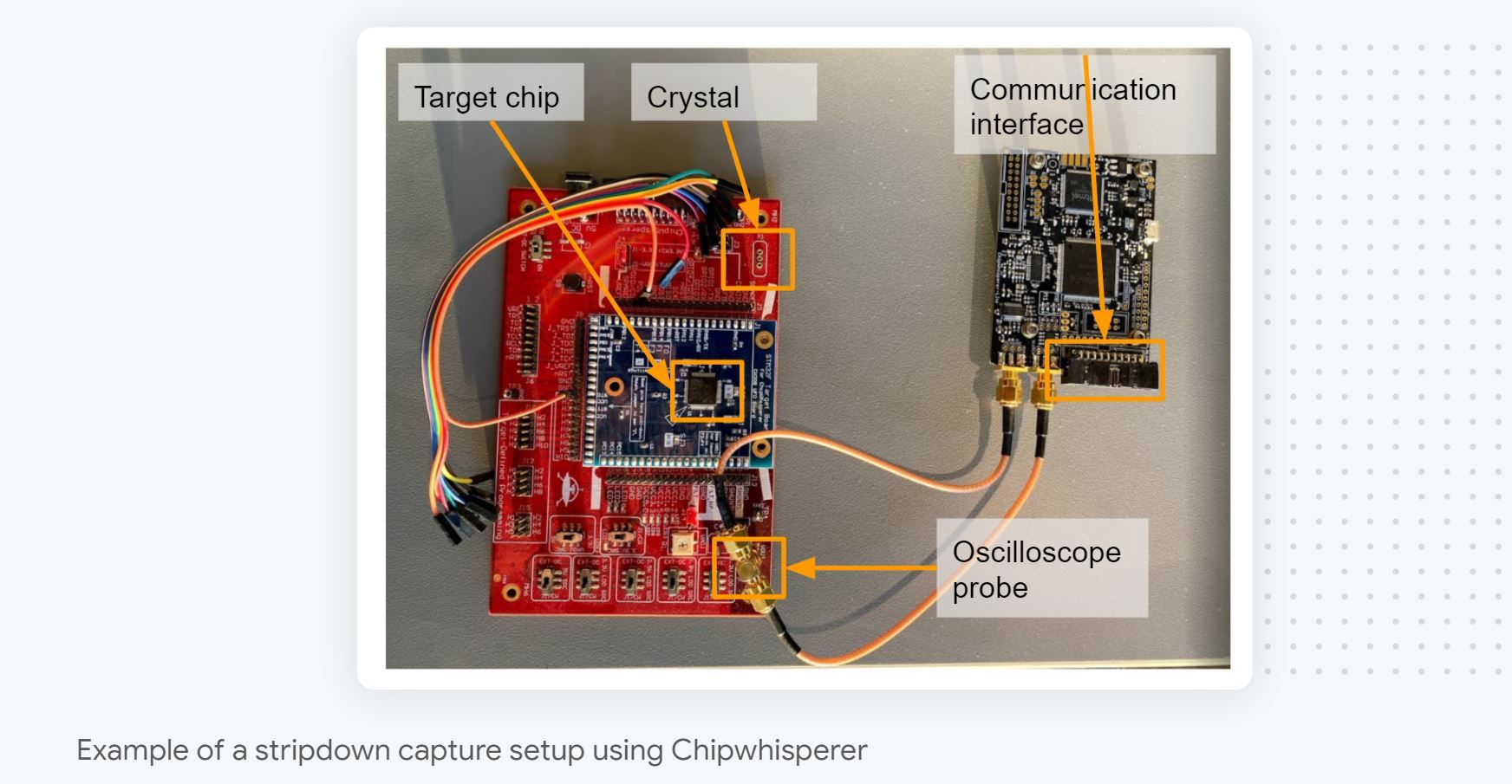
In practice, to make things easier, the code responsible for collecting the traces doesn’t directly control the oscilloscope or interact with the targeted chip. Instead, it uses dedicated hardware that standardizes those interactions and makes them easy to script. In our team, we use Chipwhisperer, as we like its Python API, affordability, openness, and diverse choice of targets (hardware architecture + crypto implementations).
For full transparency, the setup we use for research doesn’t use the Chipwhisperer integrated oscilloscope. Instead, it relies on external oscilloscopes that can capture at a higher frequency. We need this extra hardware to be able to target chips that have a high clock frequency and over-sample as we do asynchronous collection. That said, to get started, Chipwhiperer is more than enough, as many targets have clock speeds that are well within what the integrated oscilloscope can handle.
What power traces look like
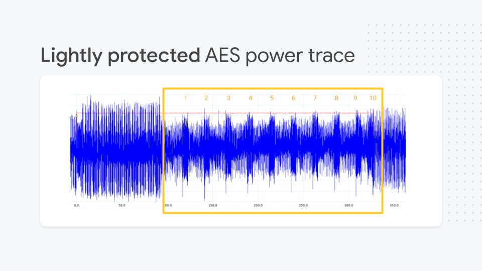
At the end of each capture, you end up with a set of power traces that looks like the one visible in the screenshot above. It shows you the power trace for an unprotected AES implementation. It is clear that this implementation has very few SCA countermeasures, as 10 rounds of AES are clearly visible. Better protected implementations still exhibit these 10 rounds pattern but not necessarily as clearly.
Usually, for SCA the numerical precision used for the recording varies between 8 and 12 bits, depending on how precise the oscilloscope is (a high-end oscilloscope can even go up to 16 bits of precision, but we haven’t needed this so far) which is why, in practice, we store the traces as unsigned char (8 bits) to save space. Even stored like this, our zipped TinyAES 65 k traces data set ends up weighing 7 GB+. Our largest research datasets, which target protected implementations, end up weighing over 1 TB, which makes training on them challenging, but that’s a topic for another day :)
Data sampling
The goal of collecting traces is to build two data sets of examples: a training one and an evaluation one. The training corpus is used by attacking algorithms, deep-learning-based or not, to learn how power consumption changes in relation to the key used during encryption. The evaluation corpus, as discussed later, is used once the algorithm is trained/calibrated to evaluate how efficient the attack is.
For the training corpus, the attacker is able to freely choose what keys and plaintexts will be used during the computation, as it is assumed that this step is run on devices that are under the attacker’s control. Having an efficient sampling algorithm is useful here, to ensure that the space is correctly sampled. The amount of trace to collect varies, depending on how protected the implementation is. As mentioned above, we tend to err on the cautious side, and usually collect over 1M traces. As a result, the process takes up to several days depending on how slow the implementation is and how large the traces are. Fear not! Hopefully, in a not too distant future, we plan to open source our datasets so you won’t have to go through this.
The evaluation corpus is different. Its goal is to represent a real target. As a result, the keys used in this corpus should be purely generated at random, as the attacker has no control over how users choose their keys. Furthermore, as we do in our research, this corpus should be generated on a different chip, to ensure that the attack generalizes across chips, as there might be slight behavioral variations due to chip manufacturing tolerance.
Synchronous versus asynchronous capture
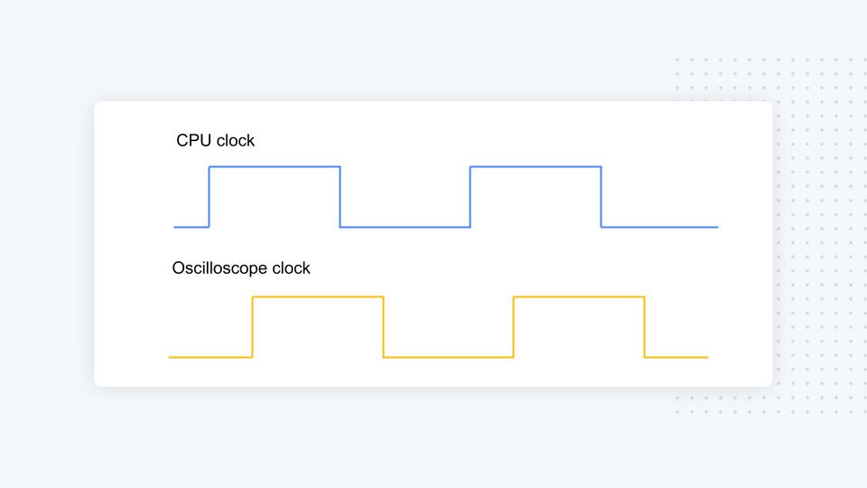
A final and often overlooked choice made at capture time is whether to perform a synchronous or asynchronous capture. Let’s briefly explain the difference between the two and when to use one over the other.
Performing a synchronous capture means that the target CPU clock output is used by the oscilloscope to align its sampling with the target CPU execution, as you can see above. This makes it possible to capture the power consumption at the target clock frequency without losing any information. This type of capture is reserved for evaluation during chip development, because in real-world settings, the attacker doesn’t have access to the CPU internal clock, as no sane secure hardware will ever expose it. In our research, we exclusively use synchronous capture in conjunction with SCALD, our deep-learning-based side-channel attacks leakage debugger, as it is intended to help chip designers to quickly find the leakage origin and fix it.
Performing an asynchronous capture implies that the CPU clock is not being used to synchronize the oscilloscope clock. As illustrated above, being asynchronous forces you to oversample to avoid missing power consumption changes. More precisely, the Shanon-Nyquist sampling theorem states that you need to sample at least two times faster to properly qualify the signal. In practice, you need to capture at least at four times the target clock speed to be safe and ensure that you have exploitable numerical traces. Asynchronous capture is the only realistic mode when evaluating attack performance, because an attacker never has access to the secure element clock. While using async collection might sound obvious, sadly, many research efforts use synchronous capture instead, because over-sampling creates traces that are four times larger, which makes them harder to store and attack. For example, some of the most protected AES implementations span over 100 K points per trace, which in asynchronous mode led you to capture 400 K points. Processing examples of that size using deep learning is quite challenging, as it’s very taxing on the GPU memory. However, it is not impossible with the right neural network…
As an aside, over-sampling strategy is one of the key points where electro-magenetic side channel attacks (EM-SCA) differ from the power one. An EM-SCA requires significantly more oversampling. But let’s save how to perform an EM-SCA for another time, as this post is already quite long and it’s not critical to understand how things work 😊.
The training phase
The training phase is performed on a computer under the attacker’s control and is meant to build a leakage model using the traces collected earlier. Traditional SCA techniques, such as template attacks and SCAAML (side-channel-assisted with deep learning) attacks, both use a “training phase” to learn those patterns, but the way they go about it is very different: Template attacks, which are state-of-art attacks prior to deep learning, use training data to perform a multivariate statistical analysis, creating an approximate leakage model known as the Hamming Weight Power Model. SCAAML attacks use raw training data to train deep-learning models that can predict a targeted value directly from it. In a way, this is very similar to what happened in the computer vision field: Template attacks, like old vision algorithms, rely on human crafted features, while deep-learning models work directly with the raw data.
In this tutorial, I am not going to cover how to perform template attacks in detail, as it’s not necessary to understand how to use deep learning for side-channel attacks. However, toward the end of this post, I will discuss why deep learning is better than template attacks. If you are interested in learning how to perform a template attack, you can check out this paper and the Chipwhisperer tutorial on the subject.
Attack points
The next question we need to answer is: What values should the attack predict? The obvious answer would be the value of the key bytes. However, in practice, for most implementations, this won’t work unless by mistake you included the load of the key in memory in your capture. I call this a mistake because, in most real world scenarios, the key is baked in the device and only loaded once, not at every encryption, so expecting to observe it with every encryption is an unreasonable threat model and leads to false positive results.
Instead, the attack tries to predict the values of what are called attack points also known as (leakage) sensitive variables in the cryptanalysis community. In a nutshell, an attack point is a point in the algorithm where the computation did cause some memory change (changing a register value, setting a value…) that has some relation to the value we try to recover (e.g XORing it). Changing the memory values triggers a power consumption change, which means that this change will be observable from the power trace.
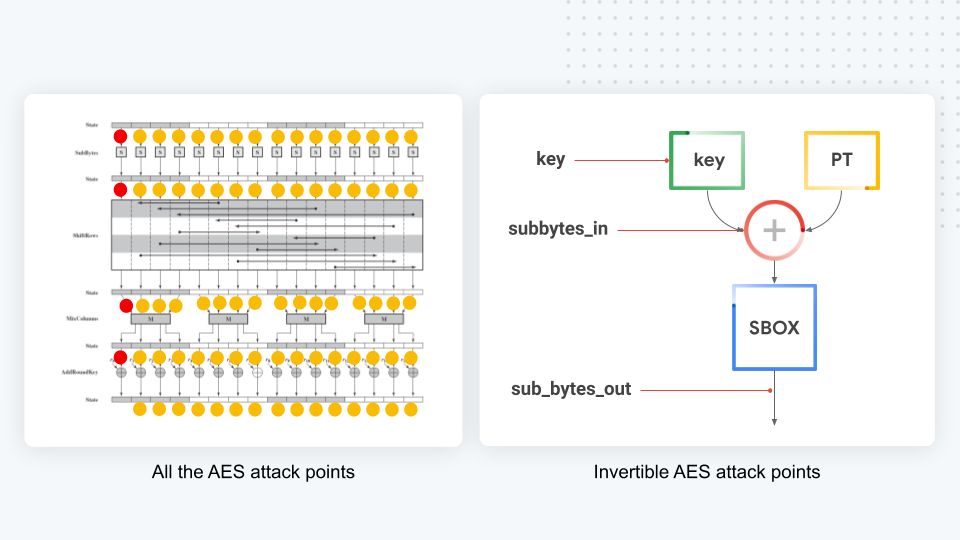
As you can see in the diagram above, which depicts AES operations overtime, AES has many attack points throughout its 10 rounds (attack points are represented by the red/yellow dots). However, in practice, most of them are non-invertible—we can’t infer the key byte value from the guessed value. As a result, we focus only on the red dot ones, which are directly invertible. The three main ones, all located in the first round and depicted on the right side of the diagram, are:
- key: The obvious one—trying to infer the key as the byte value is stored in memory. Most likely to fail, but you never know! It can’t hurt to test. :)
- sub_bytes_in: The value of the targeted byte after the key is stored with the plaintext.
- sub_bytes_out: The value of the byte after it was substituted for another value using the AES BOX.
How easy it is to attack one point over another is implementation dependent. For TinyAES, both sub_bytes_in and sub_bytes_out are easy to attack and key, as expected, doesn’t work.
Model design
As mentioned earlier, in our experience, both RNN- (recurrent neural network) and residual CNN- (convolution neural network) based architectures can give good results. However, we also found out the hard way that it’s often hard to find the right architecture parameters, which is why we rely heavily on hypertuning to find what works for a given target. That said, for this tutorial this won’t be an issue, because, through repeated testing and refinement,we came up with a model architecture that consistently works very well on easy targets. For those curious about more detail: It’s based on the pre-activation form of ResNet (aka ResNet v2), a popular architecture for machine vision.
Once you find the right model architecture and the right hyper-parameters, the model training procedure is very standard. The only two things worth noting are:
-
Inputs must be scaled or the models won’t converge at all. We scale inputs between -1/1 but 0/1 should work as well.
-
The output layer must use a softmax activation and you should use categorical cross-entropy as a loss function. Beside being the best way to converge the network, using a softmax activation is mandatory to carry out the attack because it ensures that the network outputs a probability distribution over all byte values that are possible outcomes as discussed in the next section.
The attack phase
As a last step, the trained model is used to recover keys that were not seen during training to evaluate the attack effectiveness. The attack data set is a little different from the training one, as the keys used in it must be drawn in a purely random fashion to mimic the fact that in real world settings, device keys are generated at random when they are initialized.
How are keys recovered from the traces?
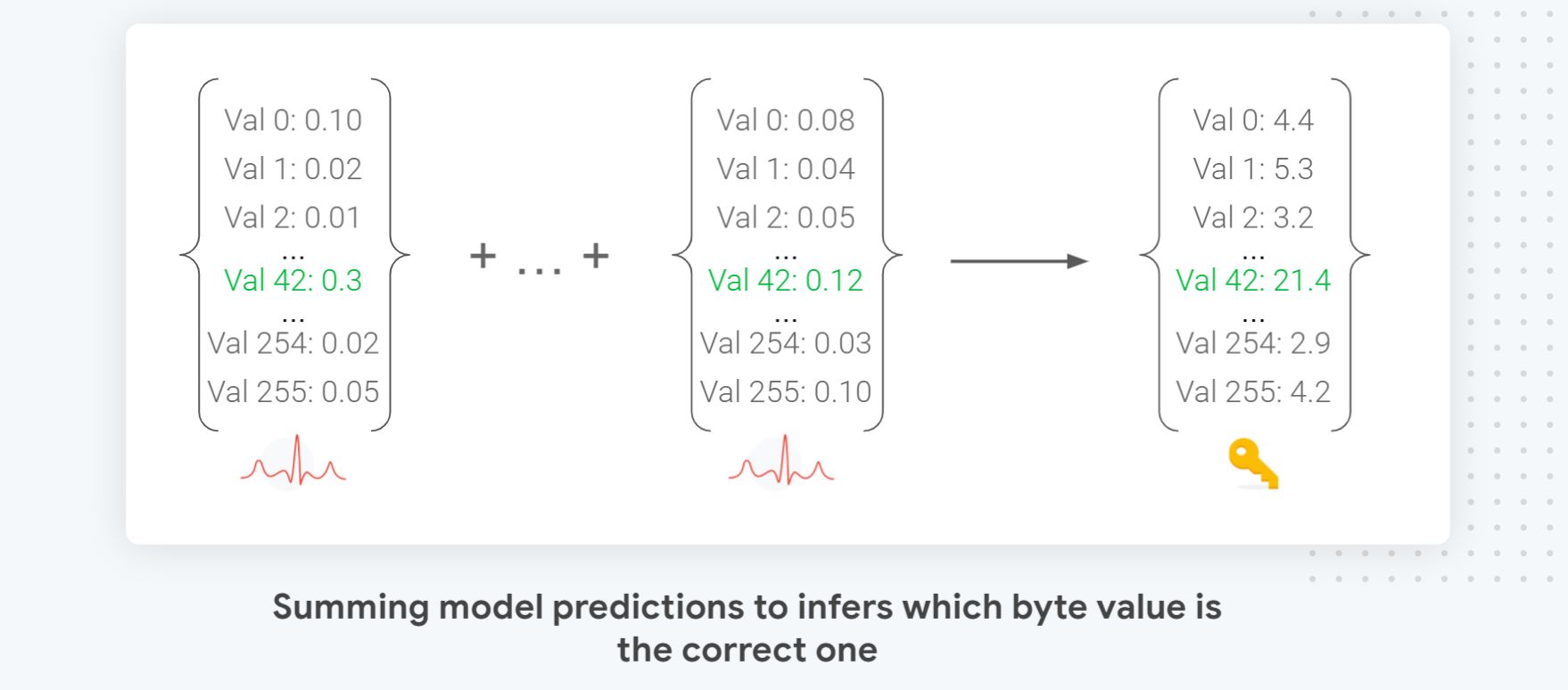
As alluded earlier in the post, one of the key advantages of using deep learning for SCA is that it makes it easy to perform a probabilistic attack that scales in the number of traces used. You simply need to accumulate the Models’ predictions, as seen in the diagram above, to decide which byte value is the most probable. This direct summing means that the more traces you combine during the attack, the more evidence is accumulated, and the better your success rate will be, as long as your model did converge (aka it predicted more accurately than random).
This attack formulation also has the advantage of naturally producing a fully ordered list of potential guesses which makes adding a brute-force component to it to test the most likely combinations across the 16 key bytes trivial. Last but not least, it allows us to know how far the correct guess is from the top which allows us to measure attack improvements and compare attack models more finely.
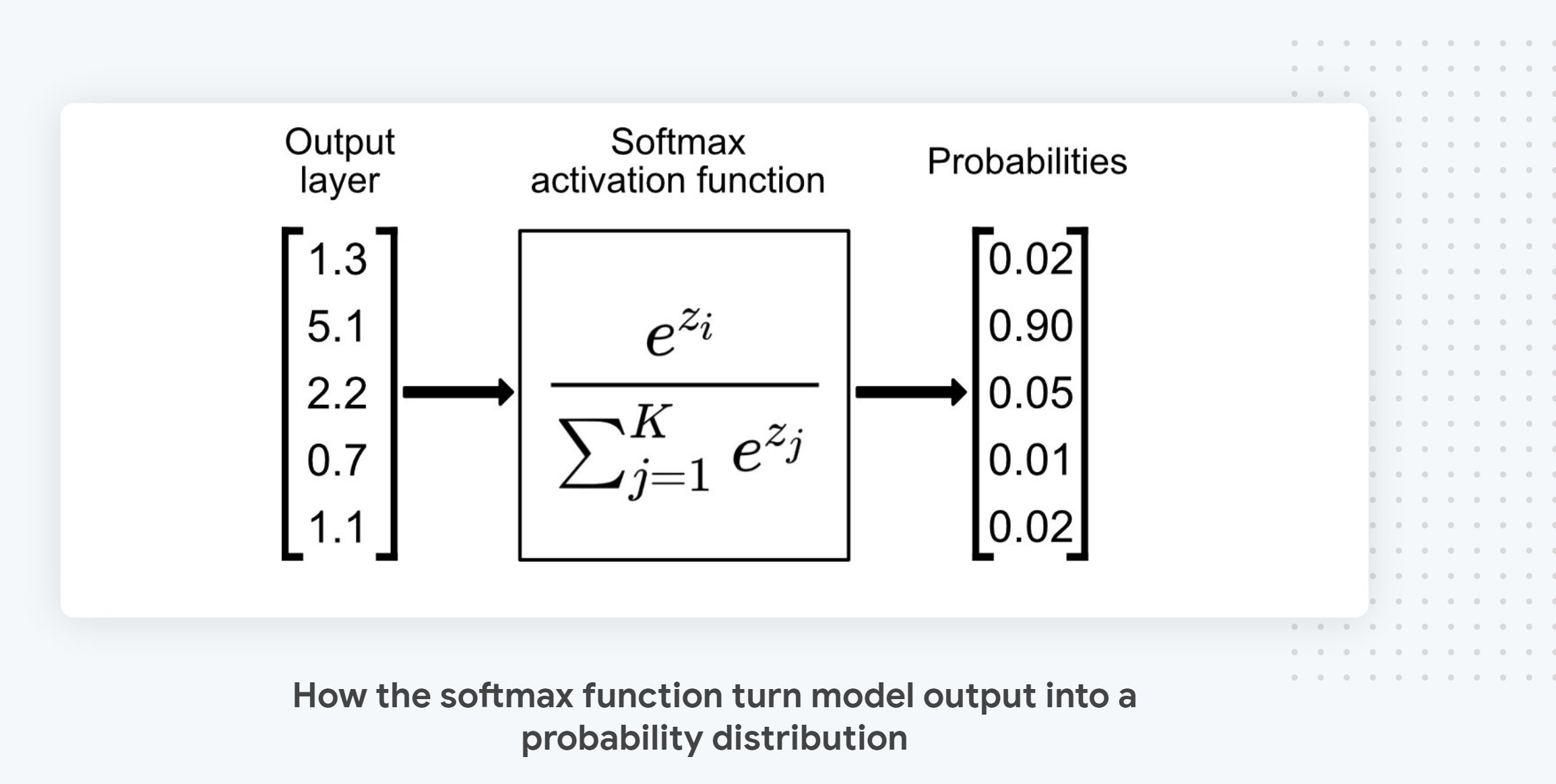
Technically, the reason why direct summing works is because the model output layer, the one that emits the predictions, uses a softmax activation that guarantees that the model output is a probability distribution over all the inputs and that its sum is exactly 1 as visible in the diagram above that illustrates how softmax works.
Finally, it is worth noting that, in practice, to deal with numerical errors, we don’t accumulate probability by multiplying them but instead, we sum their logs. This doesn’t change the attack flow, and the tutorial code implements this type of summing, but it’s an important subtlety to consider if you decide to write your own implementation.
Assessing success
The way side-channel attacks effectiveness is evaluated is a little different from algorithm cryptanalysis, so let’s contrast the two.
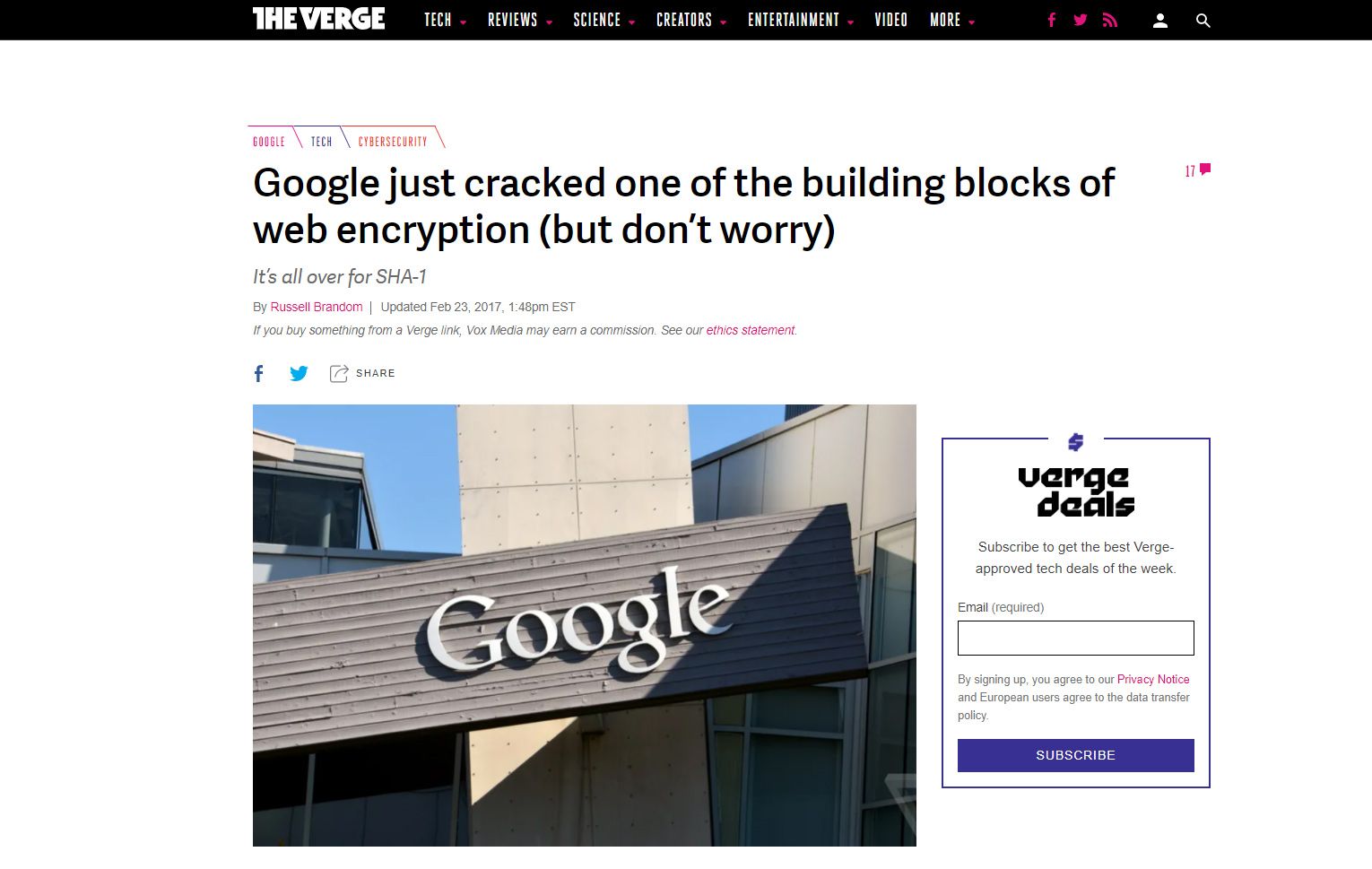
Algorithm cryptanalysis attacks are evaluated based on how much they reduce the computational cost of breaking the algorithm. For example, in 2017, we were only able to compute the first SHA1 collision because cryptanalysis techniques were allowed to reduce the computation cost from 2 80 down to ~263 . An algorithm is considered secure as long as the computational cost of performing an attack is not technically feasible. For example, for SHA-1, the cost of creating a collision via brute-force is 12 M GPU/years (impossible to do), whereas the cryptanalysis version “only” requires 112 GPU/years (hard but doable). Note that since our initial success and Marc claiming the bitcoin bounty, there have been more recent results (2020) that improved attack efficiency drastically.
For side-channel attacks, the goal of the evaluation is to evaluate the overall cost of the attack (in equipment/development time) and how many traces will be needed to recover a given key, as it is broadly accepted, as discussed earlier, that any hardware/algorithm implementation is vulnerable to side-channel attacks to a certain extent.
The number of traces needed to recover a given key can be evaluated in multiple ways, including:
- Worst case scenario for the implementation: What is the minimal number of traces needed to recover the key?
- Average case: On average, how many traces are needed to recover the key?
- Best case scenario: How many traces are needed to recover all the keys?
- Cumulative success rate: This metric can be thought of as the area under the attack curve. This is a good metric for benchmarking attacks, but it is not very intuitive to understand.
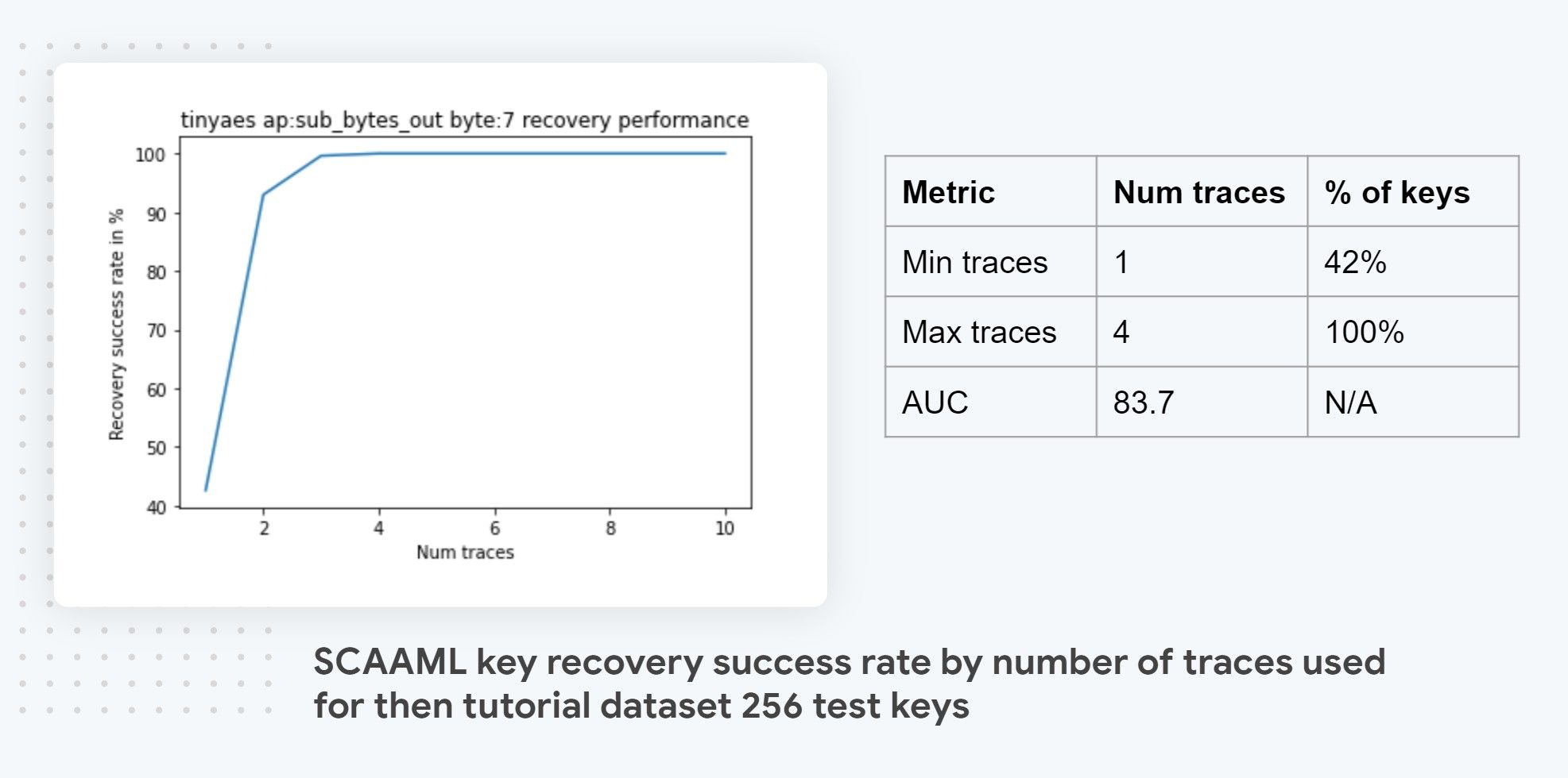
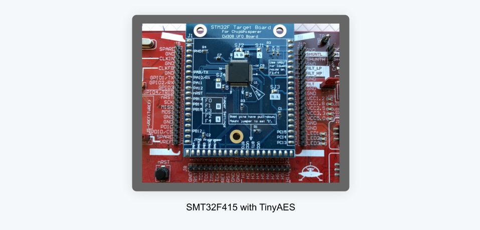
For example, for our tutorial target TinyAES on a SMT32F415 CPU, as visible in the diagram above, the worst case scenario is 4 traces and the best case scenario is single trace which are results that would be very hard to achieve with standard SCA techniques. Note that we also report the AUC which is a modified area under-the-curve metric that represents the success rate as a function of the number of traces used. It’s the single most important metric when comparing side-channel attacks because it summarizes in a single number how good and data efficient an attack is which makes comparaison straightforward. The perfect attack would have an AUC of 1 which would mean 100% of the keys are guessed with a single trace. In practice that won’t happen so instead what you are looking for is attacks that have the steepest curve / have as much area under the curve as possible as they are the one that exploits the leakage the best.
If you can’t wait and want to see how we perform the attack and compute those metrics in practice, you can take a look at the last few cells of the key recovery jupyter notebook that I will explain in detail in the part 2 of this guide.
Before concluding the first part of this tutorial, I would like to highlight a final benefits of using deep-learning based attacks: the fact that they provides us with a complete ranking of how likely each byte value is to be the correct one allows to compute many interesting additional metrics, such as how many correct values are in the top five predictions or what the average rank of the correct predictions is. Those metrics, which can’t be computed with traditional attacks, are particularly useful for comparing model efficiency on hard-to-attack implementations where the success rate is in the single digit range. Knowing the maximum rank of the correct key makes estimating the reduced search space size and the viability of a brute-force attack trivial. For example if the correct bytes values are always in the top 64 predictions, then the search space is reduced from 2^256 to 2^64, making it vulnerable to exhaustive search.
Outro
This wraps up our overview of how to do side-channel attacks and how deep learning fits into it. If you are still unclear about how this works out in practice, don’t worry! It will become clear when we start implementing our side-channel attack in the next post. At least that worked out for me 😀
Thank you for reading this post till the end! If you enjoyed it, please don’t forget to share it on your favorite social networks so that your friends and colleagues can enjoy learning about side-channels attacks too! I spent over a hundred hours creating this guide, and what kept me going is the hope that it would be useful to our community, so having it shared and used really means a lot to me 😊
To get notified when my next post is online, follow me on Twitter, Facebook, or LinkedIn. You can also get the full posts directly in your inbox by subscribing to the mailing list or via RSS.
🙏 A big thanks to Celine, Emmanuel, Jean-Michel, Remi, and Fabian for their invaluable and tireless feedback - couldn’t have done it without you!
A bientot 👋
