In this post, we explore how a Hearthstone player can predict which cards their opponent may play in future turns using machine learning.
At first, this might seem an impossible task because Hearthstone has a card pool of over a thousand cards, which can be combined into an almost infinite number of decks. However, as we will see, with the help of a lot of game replays, our algorithm is able to make accurate predictions because most players, for efficiency, use minor variations of the same deck archetypes.
At its peak, between turns three and five of a game, our algorithm is able to predict the most probable future card with an accuracy above 95%. Here is a demo of the algorithm in action:
Following the original release of this post in 2014, I had a few conversations with the developers of Hearthstone, who called this algorithm “game-breaking”. Following their request, I agreed not to release the tool or the data to avoid spoiling the game (more details here).
A more “scientific” treatment of the main results described in this blog post is published in this research paper.
This blog post is part of my series of blog posts about applying machine learning to Hearthstone. Here is the list of posts:
- How to price Hearthstone cards: Presents the card pricing model used in the follow-up posts to find undervalued cards.
- How to find undervalued cards automatically: Builds on the pricing model to find undervalued cards automatically.
- Pricing special cards: Showcases how to appraise the cost of cards that have complex effects, like VanCleef.
- Predicting your Hearthstone’s opponent deck: Demonstrates how to use machine learning to predict what the opponent will play (this blog post).
- Predicting Hearthstone game outcomes with machine learning: Discusses how to apply machine learning to predict game outcomes.
Disclaimer: The analysis was done using replays from 2014. That being said, the results still apply today, as the core mechanics of the game haven’t changed. For the same reason, the analysis should work for any card collecting game.
Last edit This post was last edited in October 2016. The introduction was fully rewritten to reflect the current state of the research. To make the post clearer, the content was partially written and illustrations were added.
Why is Hearthstone predictable?
One of the appeals of Hearthstone is the diversity of playing styles: Players have at their disposal for building a deck over a thousand cards. In theory, this diversity allows the creation of an almost infinite number of decks.
However, in practice, the decks played have a lot of predictable structure due to the following reasons:
-
Class restrictions: About half of the cards (459) are restricted to a specific hero class. These cards tend to see a lot of play as they are among the most powerful ones.
-
Card synergies: By design, many cards work best when played in combo with other very specific cards.
-
Bad cards: Many cards are just bad or under-powered, which means that they are almost never played in competitive games. However, there are quite a few reasons to include them in the game.
-
Netdecking: Last but not least, a huge fraction of players rely on netdecking, which is using a deck made by someone else (usually a pro-player) and found online.
As a result, most decks played on ladders and tournaments gravitate toward the same deck archetypes with only slight variations (aka Teching). This makes Hearthstone’s decks both efficient and predictable.
How to exploit Hearthstone’s predictability
To predict what Hearthstone opponents have in their decks, we are going to write an algorithm designed to learn probable deck structures based on 50,000 game replays. Learning the underlying structure of the decks will be used to predict what cards are likely to be played next based on the cards already played.
One might think that a huge downside of this approach would be that it requires observing quite a few cards played in a game to make good predictions.
However, in practice, by turn two the algorithm already makes good predictions. It is able, for instance, to predict two cards that the opponent has in their deck but hasn’t played yet, with a success rate of over 50% (66.3% for the first card and 44.1% for the second card).
If you ask the algorithm to predict 10 cards that the opponent has in their deck, it will get 23% of them right. This is fairly impressive given that these are predictions based on seeing only one or two played cards.
As the game progresses, the algorithm will get an even better sense of what the opponent is playing and the prediction accuracy will increase. The accuracy peaks between turns 3 and 5, where the algorithm is able to predict the most probable card the opponent has in their hand but hasn’t played, with an accuracy above 95%.
Before delving into the results more, let’s backtrack a little and look at how the algorithm works.
##Algorithm’s objective
At a very high level, the algorithm we are developing needs to do two things:
-
Retrieval: Given the opponent’s class and the list of cards that they have played so far, it should return a list of cards that the opponent is likely to have in their deck but hasn’t played yet.
-
Ranking: The returned list must be ranked by the probability of the cards being in the opponent’s deck. Ideally, we want the first card of the list to be the one that has the highest chance of being played in future turns, the second one to be the second highest and so forth.
In computer science jargon, we call such an algorithm a machine-learning ranking algorithm.
Algorithm overview
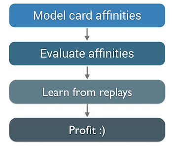
As visible in the diagram, to build our prediction algorithm we need to:
- Model the relationships between cards so the algorithm has the structure necessary for learning the “shape” of decks. Note that we build one model per class because each class has some cards that are unique to it.
- Build a scoring function that, given a set of cards, returns the most probable cards in the deck based on how the cards are related to each other.
- Train our algorithm on a set of game replays so it can learn the shapes of the decks and relationships between cards.
- Evaluate our algorithm to see if it works, tune it and generate a probability table that will tell us how accurate the algorithm is at predicting cards for a given turn.
##How can we model relationships between cards?
Modeling the relationships between the cards is the main difficulty we have to overcome in building our prediction algorithm. Finding the best way to represent which cards are usually played together is a delicate balancing act.
On one hand, you want to capture only meaningful relations to avoid making inaccurate prediction (aka “undercutting”). On the other hand, you don’t want to be too strict (aka “overfitted”) and be able to handle gracefully the slight variations between decks and the game’s inherent randomness due to the order in which cards are drawn and sequenced.
I will spare you my unsuccessful attempts with various models and focus on the one I ended up using: a variant of the n-gram representation. This model is probably the simplest representation you can use, but because of its simplicity it is also very robust.
That n-grams are the best representation is only half surprising since the method was developed by Shannon, one of the fathers of computer science, to predict elements of the English language based on statistical modeling and, therefore, it needed to be very robust.
The original paper on n-grams is called Prediction and Entropy of Printed English. It is one of the best papers I have ever read — it is brilliant, understandable and inspiring. If you have any interest in computer science, I highly recommend that you read it. It is well worth it.
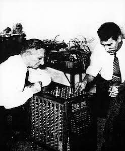
Amusingly, as visible in the photo, Shannon was also deeply interested in using algorithms to play board games. This led him to write a groundbreaking paper on artificial intelligence in 1950 on how to get computers to play chess.
How n-grams work
Okay, enough history! Here is how n-grams work. An n-gram is a contiguous sequence of n items from a given sequence of items. In our case, the n-grams are sequences of cards. We usually work on sequences of two items (“bigrams”) or three items (“trigrams”), though some algorithms use 5-grams or even more, especially for natural language processing.
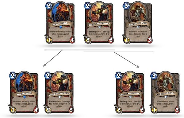
In our case, we will stick with bigrams and trigrams. Extracting the sequence of bigrams for a list of three played cards is illustrated above. As you can see, it generates two pairs of cards that were played consecutively.
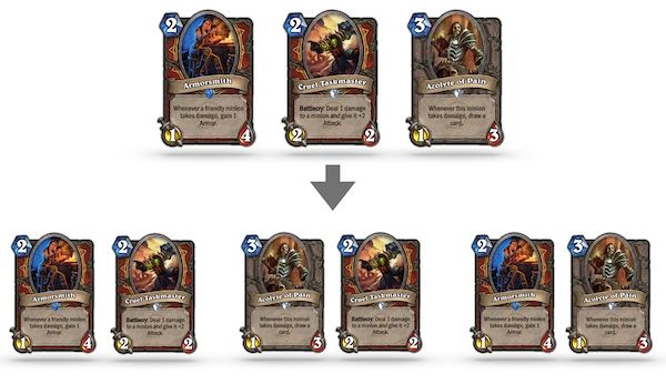
As mentioned earlier, we are going to use a slight variation of the traditional n-gram model, as we are going to extract a bag of bigrams and trigrams. As illustrated above, this means that instead of extracting only the pairs of cards that appear one after another, we will extract all possible pairs of cards regardless of their order. The reason for relaxing the contiguous constraint is twofold:
- It models that cards are drawn at random.
- It accounts for the fact that the order in which cards are played in the same turn most often has no impact, which leads players to use them in an arbitrary order.
The algorithm learning phase consists of processing the replay of each game, extracting the sequence of cards played by the opponent, and extracting a bag of bigrams and a bag of trigrams from this sequence of cards.
Then all those bags of bigrams and trigrams are summed, so that at the end of the training phase, the algorithm knows how often the cards in each pair or triple are played together.
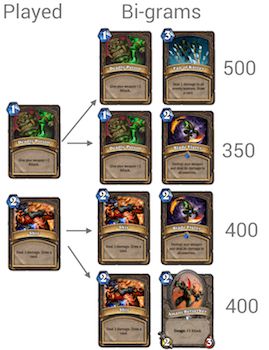
For example, as depicted in the figure above, the algorithm can learn that the combo Deadly poison/Fan of knives is a very popular Rogue combo as the two co-appear in 500 games.
How can we predict upcoming cards?
Now that our algorithm has learned the relationships between cards, to create our predictions we need to combine the frequency ranks.
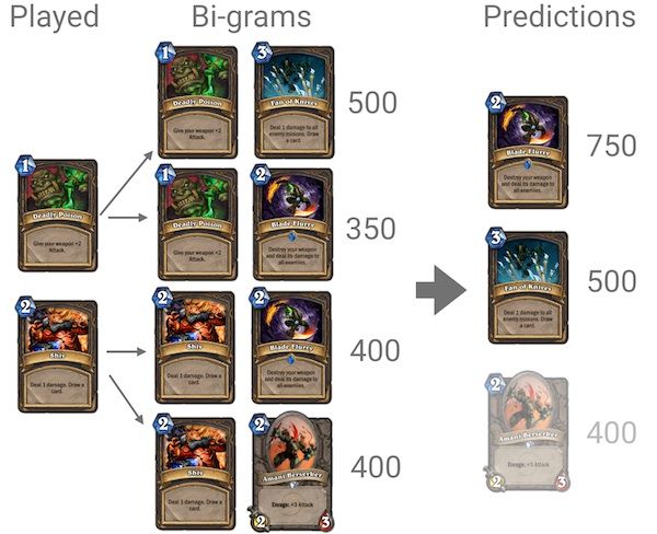
The easiest way to explain how we do this is with an example. Assume that our opponent, as shown in the figure above, has so far played the cards Deadly Poison and Shiv.
What the algorithm will do is look at all the pairs of cards that contain Deadly Poison and all the pairs that contain Shiv (middle of the figure) and retrieve from this a count of how frequently each card was seen with the other (step 1). In our example, Blade Flurry was seen 350 times with Deadly Poison and 400 times with Shiv. Fan of Knives was seen 300 times with Deadly Poison and Amani Berserker was seen 400 times with Shiv.
The algorithm then sums all those counts and sorts the cards by this count (step 2). In our example, Blade Flurry ends up as the most seen/probable card with a count of 750, Fan of Knives is second with a count of 550, and Amani Berserker is last with a count of 400.
Next, the algorithm orders the cards by the count (step 3). It then simply returns the cards with the highest counts and excludes cards with a count that is too low (here, Amani Berserker).
Technically, we normalize (softmax) by the total count to display a percentage, but this does not change the core principle, so I removed that step from the diagram for clarity.
Data, data, data
To work, our algorithm requires a lot of game replays. Experimenting with various dataset sizes, I started to get consistent results when using over 10,000 game replays. Moreover, using more than 50,000 games does not improve the results, so I settled for a dataset of 50,000 replays that were played between May and July 2014.
The main painful point at that stage was getting the replays and processing them. I converted them into a game structure, which told me what cards were played at which turn and by which player.
One caveat about the dataset: Because Blizzard does not offer a replay feature, the replays were directly collected from various players and, therefore, we don’t know what cards the opponent drew. We only know what cards the opponent played. This not an issue, as it reflects the real game conditions under which we want the algorithm to operate, but it is worth mentioning.
Algorithm evaluation
Now that we have an algorithm and data, all that is left is using the algorithm and seeing how well it performs!
I must confess here that it was not that simple. Inadvertently, I introduced a very subtle bug that made the algorithm behave erratically and under-perform, and it took me a while to find and fix it (it turns out that debugging machine learning algorithms is not that easy :)).
Anyway, once everything was working, I evaluated the accuracy of the algorithm by training it on 45,000 games, keeping 5,000 for testing.
Prediction accuracy
The first way to evaluate the algorithm is to evaluate how often a card predicted to be in the opponent’s deck ends up being played by the opponent at any later point in the game.
To answer this question, I looked at the top 10 predicted cards on each of turns 2 through 15, as returned by the algorithm. I then looked at how often these predicted cards were played.
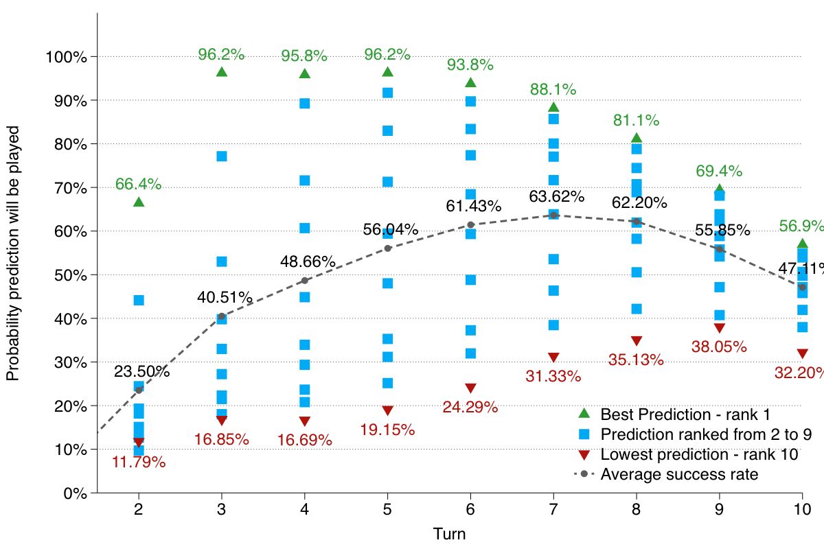
As visible in the chart above, the algorithm works very well! For example, the card that the algorithm believes is the most likely to be in the opponent’s deck on turn 5 is eventually played by the opponent 96.2% of the time. The second most likely card ended up being played 91.69% of the time, etc.
Ranking accuracy
Looking at the graph above, we also observe that the ranking function performed as expected: the highest ranked card ended up being the card that was played the most often. Similarly, the lowest ranked card is the one that is the least often played.
Evolution over the turns
It is interesting to look at the trade-off between having more information as more cards are played and there being a smaller pool of cards to predict from as the number of cards in the opponent’s deck decreases.
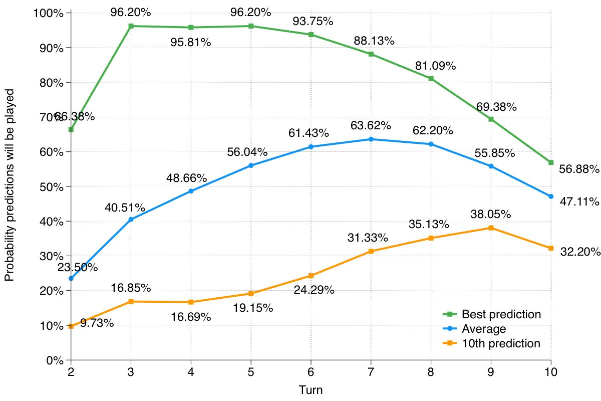
As captured in the graph above, the best prediction of the algorithm is when it hits the sweet spot of having a lot of information and a lot of cards to predict, which is between turns 3 and 5. After this, the best prediction accuracy steadily decreases.
On the other hand, seeing more cards keeps increasing the average accuracy of the algorithm, till turn 9, since the predictions ranked between 2 and 10 becomes more accurate.
Let me wrap up this post by saying that I also experimented with larger n-grams like trigrams, but the results weren’t as good, probably because they over-constrain the space.
The next post in this series tackles the problem of predicting game outcomes using machine learning.
If you want to be notified when the next post is online, follow me on Twitter, Google+ or Facebook.
You can also get the full posts directly in your inbox by subscribing to the mailing list or the RSS feed.
